[pdf]
[ps.gz]
flame
Results of flame propagation simulations with RFG method and cell-centered convection scheme
Andrei Smirnov
West Virginia University
All the results and visualizations presented here are done with the stand-alone software developed at WVU.
Introduction
The effect of turbulence on flame propagation may be due to intersections
of wrinkled flame surfaces and engulfment of unburnt regions inside the
burnt regions. This effect can be qualitatively checked using computer
simulations of a turbulent flow-field by spectral method and computing a
simplified combustion process in this flow. In this work we use the RFG procedure and a
newly developed convection/diffusion solver to test this effect.
Turbulence model
The solution for a turbulent flow is given by the following
equations (Kraichnan, 1970):
where ,\tau are the length and time-scales of turbulence,
\varepsilonijk is the permutation tensor used in vector product
operation, and N(M,\sigma) is a normal
distribution with mean M and standard deviation \sigma. Numbers
kjn, \omegan represent a sample of n
wavenumber vectors and frequencies of the modeled turbulence spectrum
|
|
|
E(k)=16(((2)/(\pi)))1/2k4\exp(-2k2)
| (5) |
A way of generating random flow-field with this method, which
represents a simplified spectral technique, is covered more in detail in
(Get a pdf-copy of the
paper).
Combustion model
A convection/diffusion solver was written to solve for the transport of a
scalar variable in a turbulent flow field generated by the RFG procedure above.
A scalar variable used was allowed to change between 0.0 and 1.0 and
corresponds to a progress variable P of a premixed combustion reaction.
For a qualitative test of the effect of flame-front acceleration due to
turbulent velocity fluctuations a simple combustion model was used, where the
progress variable in each cell was updated every time-step according to the
following criteria:
IF (P>R) P=1.0
where R is an ignition limit that was set to 0.5 in this
qualitative study. In the absence of turbulence (quiescent flow field)
the flame propagation velocity was determined entirely by the diffusion
rate constant D and in the absence of diffusion, i.e. D=0,
the flame front propagation velocity was 0. When the turbulent velocity
perturbation were introduced the flame front started propagating,
engulfing the unburnt region.
Results
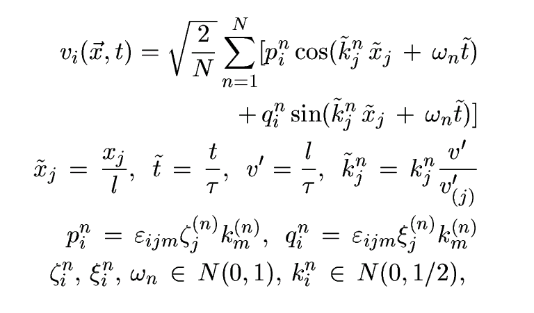
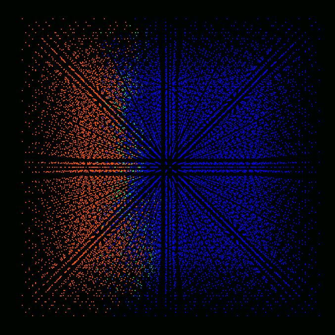
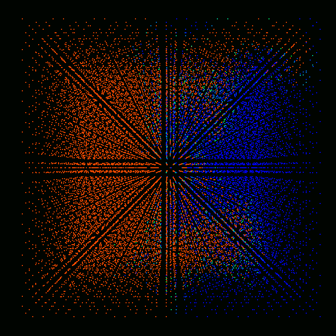
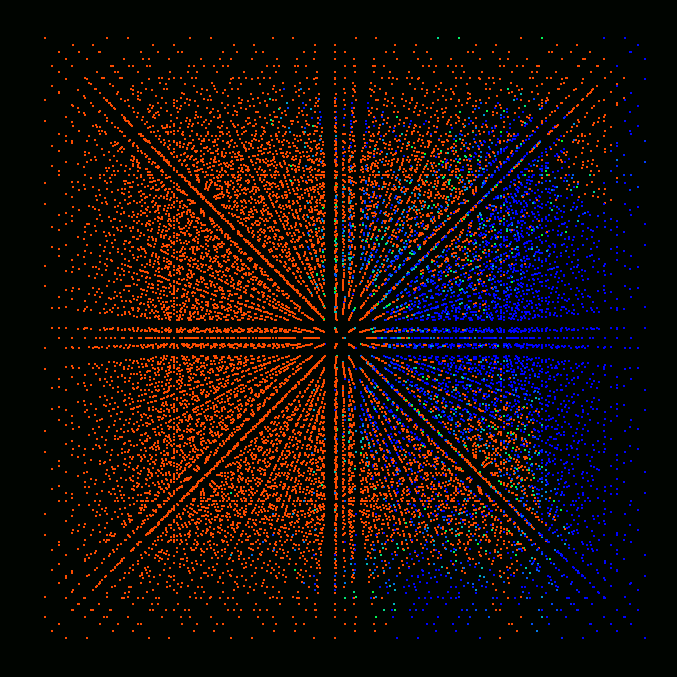
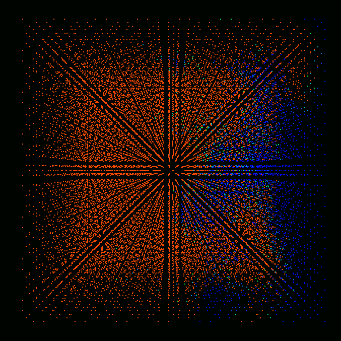
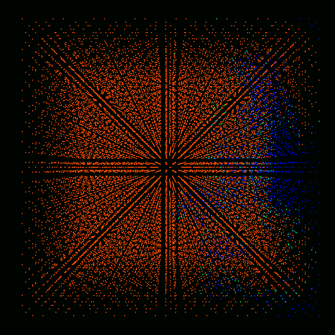
Figures below show the results of preliminary simulations of flame
propagation in a modeled Gaussian turbulent field computed on a 16x16x16
cube. Since an unstructured, tetrahedral grid is used the number of
cells in that grid is actually greater than the number of nodes,
i.e. Nnodes=16*16*16=4096, Ncells=5*16*16*16=20480. That many cells are
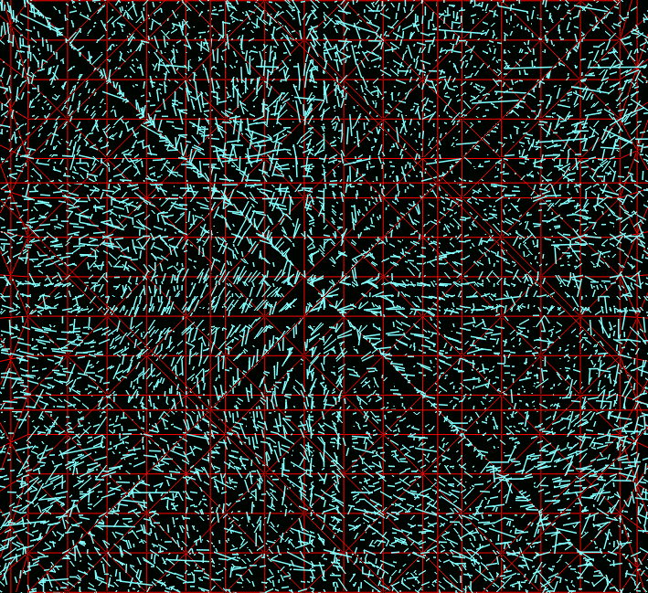
shown in the figures, each cell represented by a single colored point. Red
color corresponds to fully burnt, blue - to fully unburnt state, colors in
between correspond to partially burnt state.
Non-dimensional problem parameters:
Correlations of turbulent velocity fluctuations:

    uu=1.0
    uv=0.0
    vv=1.0
    uw=0.0
    vw=0.0
    ww=1.0

Turbulent time scale: 1.0

Turbulent length scale: 1.0

Initial distribution of P along the X-axis:

           P=1.0 for 0<X<4
           P=0.0 for 4<X<16
Computational parameters
Grid dimensions: 16 x 16 x 16
Spectral sample size: N=1000
Time-step: 0.05
where the spectral sample size parameter N refers to the equation above.
163 cube grid used in simulations.
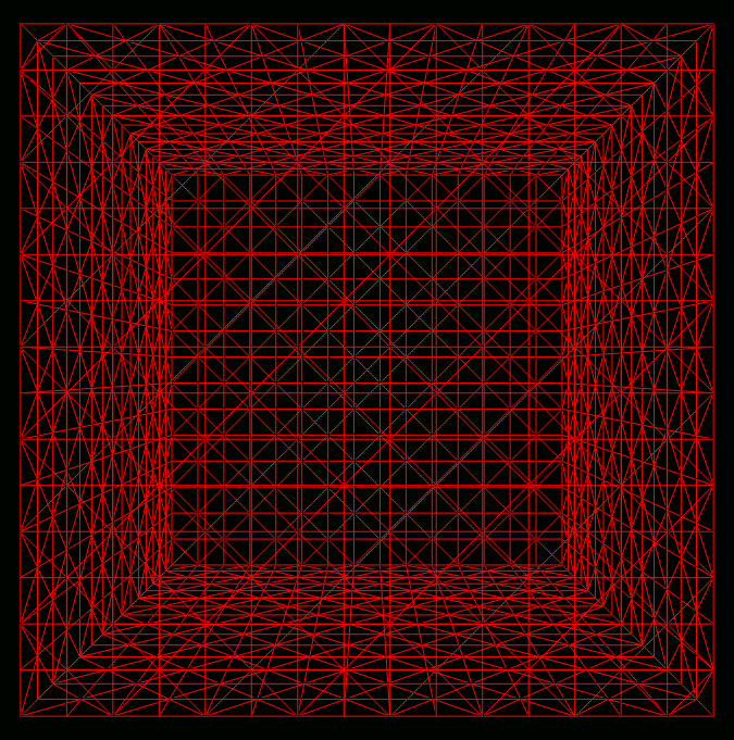
Animation of transient veolocity field (mpg)
Snapshot of turbulent velocity field generated by RFG.
Initial distribution of progress variable (concentration ratio of
burnt/unburnt species).
Time = 1.
Time = 2.
Time = 3.
Time = 4.
Time = 5.
Time = 6.
Time = 7.
Time = 8.
Conclusions
The results show the increase of flame propagation speed from 0 to
approximately 1 due to turbulent fluctuations. Formation of unburnt and
partially burnt pockets inside the burnt region is also evident from the
figures.
Acknowledgements
I would like to thank Dr. Valeri Golovitchev from
Chalmers University for the initial ideas and the inspiration needed for
this work.
The results were presented at The International Conference "Micromixing 2004" (ICMM-2004).
Abstract
[pdf]
[ps.gz]