The graphical user interface for geometric design and simulation control implemented in this work is based on Java and Java 3D, technologies as well as voxel graphics methodology.

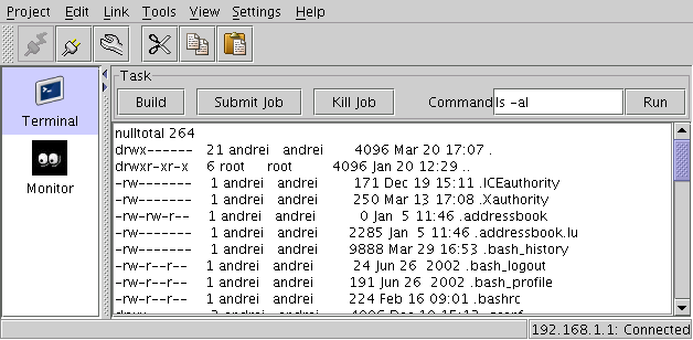
The main panel is used to start projects, setup domains, components and variables, establish and monitor remote links, and realize general settings.

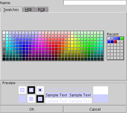
The selection of components is done by specifying their names and assigning their types. The user can also specify a color for each component for graphical display.

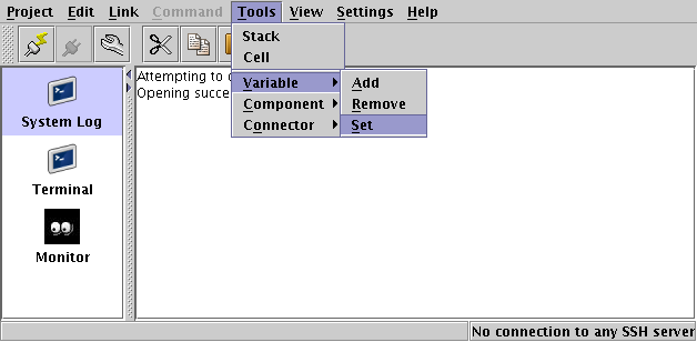
The important parameters and variables of the simulation can be setup in a variable selection/edit dialog. The dialog is invoked from the "Tools->Variables" menu.

After this selection is done from the menu, a variable table is displayed where the values for the variables can be assigned and/or changed:

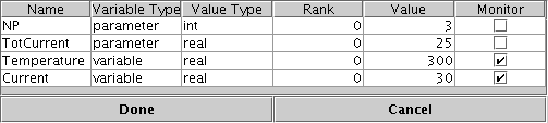
Each variable in the table is characterized by the following fields:

• Variable Type: which can be parameter or variable. A parameter has a value which is the same for the whole simulation setup (total current, convergence criteria, etc.). A variable can have different values for different components and spacial locations (Temperature, Pressure etc.).
• Value type: which can be int or real.
• Rank: 0 - scalar, 1 - vector, ... n - n-th rank tensor.
• Value: a numerical value of the variable.
• Monitor: true if the variable will be monitored and displayed during the simulation, and false if not.

The geometric design philosophy pursued in this work is based on voxel graphics. A specialized voxel graphics processor was developed by within this project to enable web-based creation of various geometric designs.

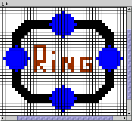
Setup of domains is realized by using 2D/3D drawing tools and 3D interactive display.

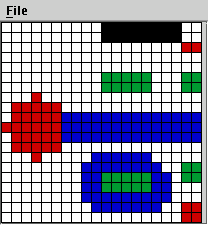
A 2D drawing tool works as a simple paint program. It enables the specification of domain components on a single cross-sectional plane of the 3D domain.

The control panel provides controls for both the 2D and 3D drawing panel.

Separate controls on the control panel enable plane selection, as well, scrolling of the plane along the domain, as well as simple plane-to-plane copying operations.

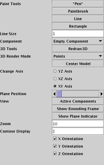
Currently implemented functions include

1. Paint tool selections. These include: Pen, Paintbrush, Line, and Rectangle. For the paintbrush and line tools the line thickness can be specified. Lines created with the Paintbrush and Line tools have 3D thickness, i.e. they are represented by a 3D objects, which can be viewed in a 3D View panel using the Redraw button on the control panel.
2. Component selection is used to select the active component to construct.
3. 3D Rendering modes include: Atoms, Wireframe, Mesh, Surface, and Points.
4. Controls for the orientation and position of the drawing plane.
5. Selection of active components to view.
6. Displaying of the bounding frame, and the position of the drawing plane in a 3D View window.


3D View panel with the active Bounding frame and drawing plane indicators.


Drawing plane tool corresponding to the 3D View above.
7. Zooming function for the Drawing panel. Zooming in the 3D View area are realized with mouse motion with the right button pressed.
8. Contour display controls used in the Wireframe view mode.

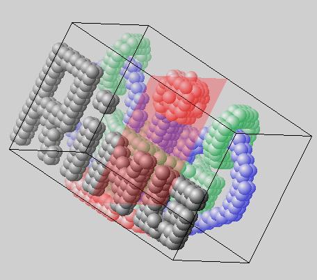
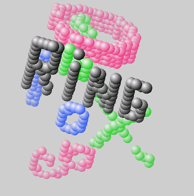
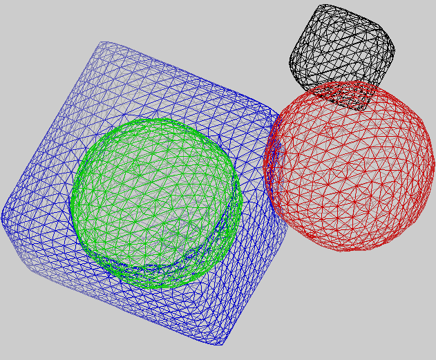
Below is an example of 3D view of a complex domain consisting of several components.

Click here for an interactive 3D view (java-applet)

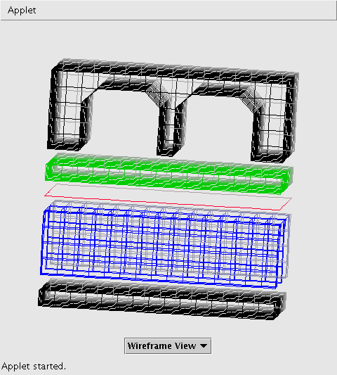
3D Viewer offers the following rendering modes:

• Points
• Atoms
• Wireframe
• Surface

The models are selected from the separate selection window that comes up after clicking at the "Tool options" button on the main panel:

Points

Atoms

Wireframe

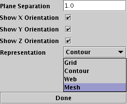
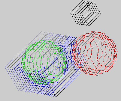
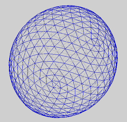
Wireframe representations include several options:

1. Contours
2. Grid
3. Mesh

1. Contour rendering is done by a set of contours around the slices of the domain by simple plane cuts: [Contour surface rendering]
   
   

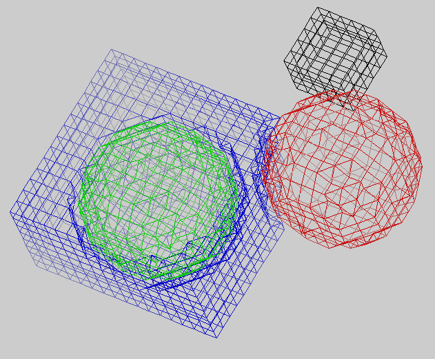
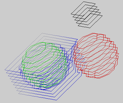
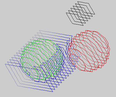
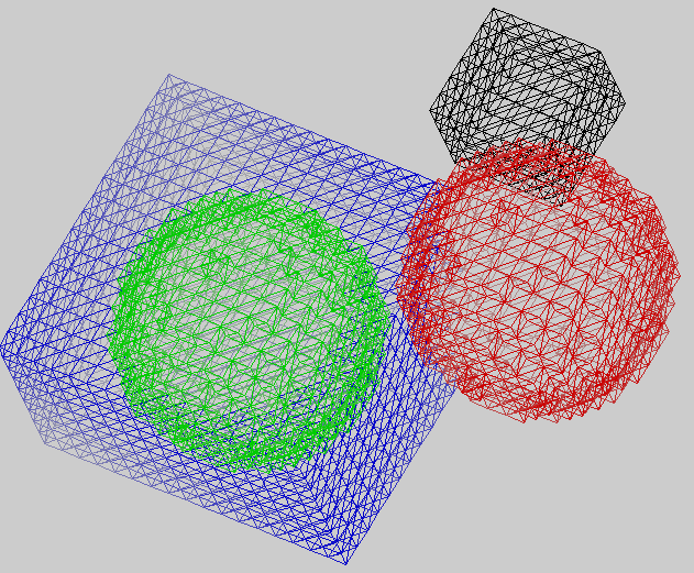
   Thus the figure above is produced by the combination of three sets of contour lines shown on the three figures below:

   [X,Y,Z contours]
   
2. Grid rendering is done by a different method whereby a triangulated mesh is created around the boundary nodes of each spatial component. [Raw triangulated mesh]
   
3. Mesh rendering is a generalization of the Grid rendering where the nodes of the mesh do not necessary include each node of the underlying pixel grid. This method is preferred when the size of the pixel grid becomes to large.

Surface

Surface rendering provides rich realistic features, such as lighting, textures, etc. Surface rendering is done in a separate window, which is opened in addition to the wireframe window, thus allowing to render both view simultaneously.

[Snapshot of the surface rendering window with a view of a fuel-cell model]

---

Surface Smoothing

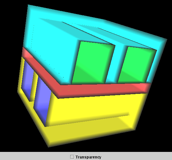
Since the objects are produced on a rectangular array of cells, the raw surface that comes out of the meshing algorithm may look rigid. A special smoothing algorithm was implemented to produce smoothing if it is desirable:

[Smoothed triangulated mesh]

Surface elasticity model is one of the plug-in models. As all the plugin models it's invocation consists of two steps: initializer and iterator. The initializer of the model remembers the surfaces of all the active. The iterator inflates the surface as if it were an elastic membrane. The initializer function is called when the rendering mode is selected. The iterator is executed each time the Inflate button is pressed on the control panel.

[Inflated boundary mesh]

Data formats

Dumping the triangulated surfaces in a generic FEM format is done automatically when the project close- or exit- menu items are selected.

Examples

A contour surface of a simple cross-flow fuel cell-type geometry is show below:

Wireframe representation of a fuel-cell
Click here for an interactive 3D view (java-applet)

3D interactive viewer allows to see all the domain components in a 3D representation. The example here demonstrates the capabilities of the viewer to represent complex multi-component systems such as fuel cells.