In the following applications the performance of the proposed particle interaction mechanism was tested in conjunction with the Lagrangian particle tracking algorithm, and a random flow generation procedure. It was applied to the cases of particle-particle, fluid-particle and fluid-particle-particle interactions.
For the purpose of testing particle interaction mechanism a three-dimensional computational grid was constructed by first generating a Cartesian grid of 32x32x32 hexahedral elements and then subdividing each element into 5 tetrahedrons, resulting in 32x32x32 nodes and 5*323=63840 elements. As the velocities of the particles were updated during the interactions the position of each particle was advanced using a second order Runge-Kutta scheme. Figure 3 shows the result of the simulated interactions of particle jets in a vacuum for different momentum-exchange mechanisms. Fig.3 shows the effect of a weak attractive potential on the trajectories of two by-passing particle jets. A slight skewness of the jet-tips arose because a the smaller attractive force was acting on the jets as they were approaching each other, and the number of particles involved in the interaction was smaller at that initial time. Fig.3 shows soft-ball type collision mechanism in case of three jets impinging at a right angle to each other. As a result of the cumulative action of the jets the original direction of each jet is changed to align with the average direction of the jets motion. Because of the elastic-type collisions in this case the momentum is not conserved. Fig.3 shows weak interaction between the three jets, resulting in a small deflection. In this case the jets remain straight until the very point of collision. Fig.3 shows a hard-ball collision type interaction when the particles are strongly deflected from original course in collisions. In this case the initially straight shape of the impinging jets is gradually destroyed in course of multiple collisions.
As can be seen from these examples a rather general types of interactions can be implemented using this technique. It should be noted though that the interaction mechanism described here is of statistical nature. In contrast to deterministic mechanisms it does not necessarily lead to conservation of exchanged quantities for each particular pair of interacting particles. It is even impossible to pinpoint the pairs of particles which interact. In this sense it is a statistical realization of a many-body interaction problem. However, the algorithm fulfills conservation laws for the whole system.
Realization of Fluid-particle and particle-particle interactions in a carrier fluid is straightforward with the fluid phase computed on the Eulerian grid in a separate cycle.
If the flow-field is produced using a turbulence modeling technique, like RANS (Reynolds Averaged Navier Stokes equation) or LES (Large Eddy Simulation) the influence of the flow on the particles results in their spatial dispersion. This dispersion is usually given as a function of the turbulent kinetic energy obtained from the turbulence model. In earlier work the authors developed a random flow generation (RFG) procedure to simulate the effect of this dispersion by generating unsteady flow-velocity fluctuations by a special procedure [{Celik et~al., }{1999}, {Smirnov et~al., }{2000}]. After this procedure is applied the particle tracking problem can be reduced to the solution of particle dynamics in an unsteady flow-filed. For this purpose we use an efficient tri-linear interpolation routine on tetrahedral elements, and additionally developed particle tracking, and particle population dynamics routines. All routines are optimized for time efficiency by using dynamically linked pointer arrays to avoid expensive loops over grid nodes or searches through the particle set.
The particle tracking algorithm was first applied to the flow-field of a bluff body wake. The LES technique was used to solve the time-dependent, three-dimensional, incompressible Navier-Stokes and scalar transport equations in non-orthogonal curvilinear coordinate system [{Shi et~al., }{1999}, {Shi et~al., }{1999}]. It is based on a domain decomposition technique, differential sub-grid scale turbulence models and second- and higher order numerical schemes [{Zang et~al., }{1993}, {Zang et~al., }{1994}].
The bubbles were injected at the two downstream corners of a square prism and convected with the three-dimensional flow-field. The flow data were given on a non-uniform grid of 80x90x20 vertexes at a single point in time. At this stage we considered only the "frozen" flow-field to thoroughly test the interpolation and particle dynamics routines. Figure 4 shows the trajectories of two bubbles injected into this stationary flow.
In the second case a ship-wake flow with bubbles was considered.
A RANS solution to the turbulent ship wake, obtained by the
researchers from Rensselaer Polytechnic Institute [{Larreteguy, }{1999}]
was used. The time-dependent fluctuating component of the flow
was generated using the RFG procedure mentioned above
[{Celik et~al., }{1999}]. A simplified equation of bubble motion was
used [{Elghobashi and Truesdell, }{1993}]
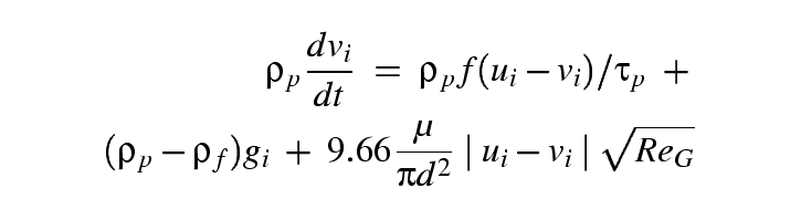
where d is bubble diameter, \rhop and \rhof are bubble density and carrier flow density, respectively, f is the dimensionless drag coefficient, ui and vi are carrier flow velocity and bubble velocity, respectively, gi is the acceleration due to gravity, ReG is the shear Reynolds number defined as ReG = ((d2)/(\nu)) ((du)/(dy)). The term on the left hand side of (3) is the inertia force, acting on the bubble due to its acceleration. The terms on the right side are respectively the drag force due to viscosity, fluid pressure gradient and viscous stresses, buoyancy and Saffman lift force [{Elghobashi and Truesdell, }{1993}]. The Basset force term was neglected, since its contribution can be considered small in highly turbulent flows [{Pan and Banerjee, }{1996}] and the added mass term was neglected for brevity in this initial stage of calculations. The integration of Eq.(3), via a second Runge-Kutta scheme provides the new velocity, vi(t), in the xi direction for each particle as a function of time. It should be noted that the RFG flow-solver and the particle solver use different time-stepping schemes with independent selection of time-steps. Usually a sub-cycling of particle iterations is required to reach a stable solution.
Figure4 shows the snapshot of a simulation where particles were injected in pulses into the wake flow right behind the ship's stern. At each time step a total of 1000 particles were injected. Although a pulsed injection is not a very realistic mechanism of particle generation, it provides a convenient way of studying the action of a random force by applying it to the initially \delta-shaped time distribution of particles. The distribution of injection locations was selected with a number density proportional to the level of turbulent kinetic energy at the inlet plane. At every time-step particle velocity was determined by the sum of the mean flow velocity and the fluctuating velocity computed using the RFG technique. In these cases the fluctuating component was added only to the particle velocities to avoid the unnecessary loops over all the grid nodes. It should be noted that this ability to use the RFG procedure only at the prescribed spatial locations offers a definite time-saving advantage in practical computations and at the same time allows to generate turbulent fluctuations at the sub-grid level. The latter qualifies the new RFG technique as a viable sub-grid-scale model.
Because of the non-uniform distribution of the turbulent kinetic energy in the ship wake particles experienced especially strong scattering in the central region of the wake and close to the injection plane. As soon as particles leave the wake region the action of the random forces ceases and particle trajectories align with the mean flow streamlines.
In another simulation (Fig.4) the bubbles were injected at a single point close to the ship hull where the turbulent kinetic energy was near its maximum. A total of 10\ 000 particles of 100 microns in diameter were continuously injected into the domain. Two seconds of real-time were simulated for the ship-length of 6m traveling with the speed of 3m/s. The figure shows the tendency of particles to agglomerate in dense groups. The characteristic sizes of these groups are in many instances smaller than the grid-cell size. This reflects the sub-grid nature of the RFG method, which enables it to capture finer details of particle dynamics than can be resolved on an Eulerian grid.
In this case we considered a case of air-bubbles rising in a turbulent water inside a square duct. This case was specially constructed to illustrate the effect of particle-coalescence. To reproduce the unsteady turbulent fluctuations the RFG procedure was used [{Celik et~al., }{1999}].
Computational grid of 32x32x64 grid nodes and 32x32x64x5=327680 elements was used to represent a vertical duct of dimensions 1x1x12 meters (Fig.5). Particles of 50µ size were injected randomly at the bottom of the duct with the velocity equal to the local fluid velocity. The particle motion was governed by (3). Particle coalescence was included as an interaction mechanism. It was given by the probability of a particle to lose its entire mass in a virtual interaction with the grid node and the corresponding probability to receive a mass from the grid node. No particle breakup mechanism was implemented at this time.
Figure5 presents the comparison of particle distributions inside the duct obtained with and without the coalescence mechanism. In all the figures the particles preserve an even distribution close to the bottom of the duct. A closer analysis of particle trajectories has shown that the initial trajectories mainly follow the buoyancy force when the particle-fluid relative velocity and the associated drag-force are small. As can be seen from Fig.5, when no interaction mechanism is given particles tend to form dense coherent streaks, especially at the upper end of the duct. This is the result of the wavy character of the fluid motions that occasionally pushes particles against the walls, creating conglomeration at the corners. As Fig.5 shows the coalescence mechanism leads to effective depletion of these regions of small particles and the formation of larger ones, which then rise faster following the increased buoyancy-to-drag force relation.
In the examples above the average number of bubbles in the case without coalescence was close to 12000, whereas in the case of coalescing bubbles only around 4500 bubbles of different sizes were engaged at any given time. These data are still of a rather qualitative nature, since the exact parameters for bubble coalescence probabilities are still to be worked out on the basis of experimental data or theoretical analysis. Nevertheless, the algorithm has shown a good performance with only about 30% increase in computational time with the interaction scheme added.
In the computations of 10,000 particles it took about 2 hours of computer time to reach a steady-state regime for the case of the duct flow running on Pentium-II (450MH) processor.